
I have been porting the h e i s h e r e reverb to Reaktor Blocks. Reaktor Blocks and Reaktor Core are a fantastic playground to explore DSP algorithms, and h e i s h e r e is an amazing ensemble by Lazyfish. It consists of a crazy sound engine, fed into a simple yet great sounding reverb. It is implemented in Reaktor Primary (it was actually built in Reaktor 2), but I wanted to port it to Reaktor Core, as Blocks are all implemented in Core.
I spent a few hours exploring the underlying formulas in Mathematica to get a better understand at what is going on. It is quite hard at times to debug / visualize the maths in Reaktor core, so I like to rewrite the patch in a more standard programming language. Mathematica still allows me to dynamically interact with the numbers, and can even apply them to audio. I heartily recommend it.
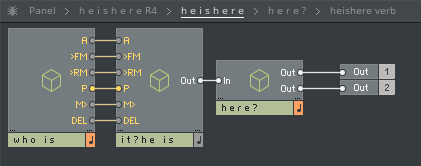
h e i s h e r e primary
h e i s h e r e structure
The basic structure is fairly simple, a sound engine (who is) is fed into an effects processor (it? he is), and finally ends up in the reverb (here?).
The structure of the reverb looks like this:
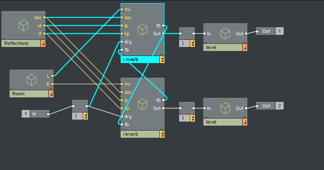
It consists of a few parameter computation macros (Reflections and Room), two feedback structures (for the left and right channel), and finally a level macro used to compress and adjust the level of the output.
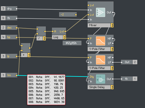
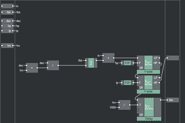
While the parameter and level macros are mono, the actual reverb is polyphonic, which is a common pattern in lazyfish ensembles. The 8-voice polyphony of the reverb modules is used to create 8 parallel delay lines, that crossfeed into each other. This is the structure of the reverb macro:
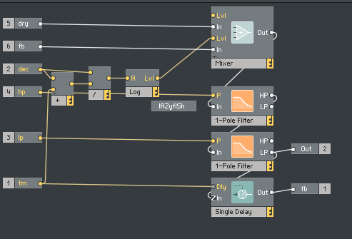
The input is mixed with the attenuated feedback level, fed into a bandpass filter (built as a HP in series with a LP filter), and finally delayed by a simple delay line. This is a common structure for the modelling of late reverberation (also called diffuse reverberation).
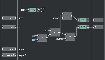
Delay length computation
The delay lengths are chosen to be exponentially spaced to achieve a dense reverberation pattern. Let’s look at how these delay lengths are computed:
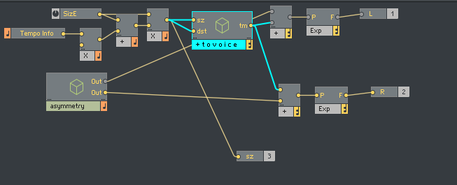
The SizE inpt is squared, and fed into a macro that spaces it out linearly. It is worth noting that the times start at twice the size, so that there is a slight effect of early reflection, since the first delay will be moving away from 0 as size gets bigger. This is a slightly untangled view into the “+ to voice” macro.
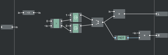
The asymmetry module can add a constant delay to either the left or right channel, depending on the polarity of the aSym knob.
Finally, the linearly (and spatially slightly offset) delay times are fed into an exponential. Looking at the computation in Mathematica allows us to see what is going on a bit better:
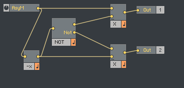
computeAsym[aSym_] :=
  {aSym*If[Not[-aSym > 0], 1., 0.],
   aSym*If[Not[-aSym > 0], 0., 1.]};

pitchToFrequency[pitch_] :=
  440. (2^((pitch - 69)/12));

computePitchTable[dst_, sz_] :=
  Table[dst + sz*i, {i, 1, 8}];

computeFreqTables[size_, asym_] :=

 Module[{asym2 = computeAsym[asym],
   table = computePitchTable[size^2, size^2]},
  {pitchToFrequency /@ (table + asym2[[1]]),
   pitchToFrequency /@ table + asym2[[2]]}]

Manipulate[
 Module[{asym2 = computeAsym[asym]},
  Grid[{
    {"asym", asym2},
    {"linear times",
     ListPlot[{#, 2} & /@ computePitchTable[sz^2, sz^2],
      Filling -> Axis, PlotRange -> {{0, 20}, Automatic},
      ImageSize -> 300]},
    {"exponential times",
     ListPlot[Map[{#, 2} &, computeFreqTables[sz^2, asym], {2}],
      Filling -> Axis, PlotRange -> {{0, 5000}, Automatic},
      ImageSize -> 300]}

    }]],
 {asym, -4, 4},
 {sz, 0, 2}]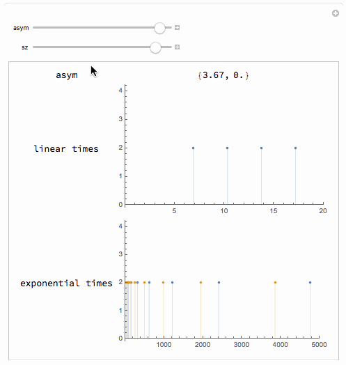
Level adjustment
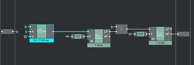
Finally, the output of the delay lines is summed, and scaled using the “level” macro.
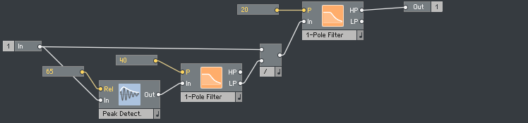
The input is fed into a enveloper follower with a relatively long release, and further low-passed using a LP filter. The input is then divided by this control signal, and high-passed to avoid DC signal and low frequencies. This has an effect similar to a compressor, and also brings the signal down into the -1 - 1 range.
Constructing the reverb in Reaktor Core
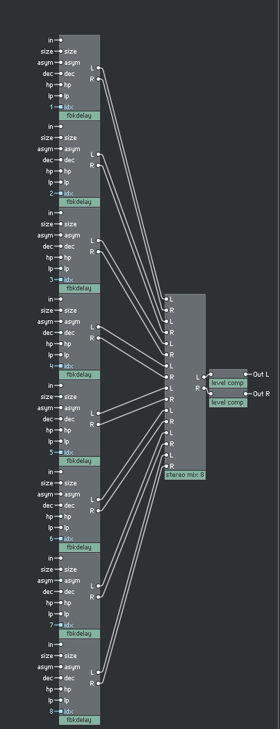
Sadly, we don’t have the luxury of polyphonic signals in Reaktor Core, so that the 8 feedback delay lines have to be wired up separately.
Since I wanted to build the reverb as a Blocks, the input settings come in as 0 - 1 values. They are first scaled up to the original values. I go for the brute force approach because it makes the structure clearer.
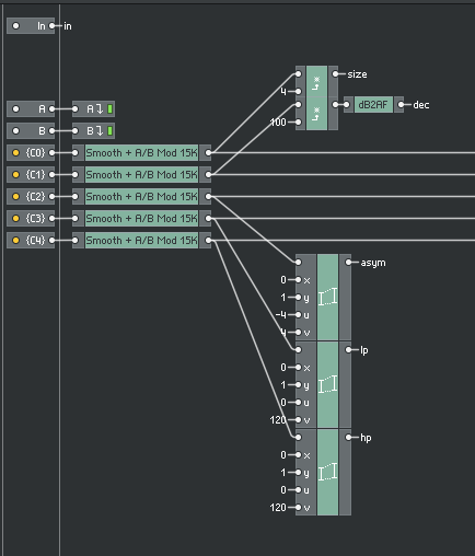
The basic structure of the core implementation is 8 delay lines, summed and fed into a level macro. This again is a bit brutish, but I tried implementing the structure using the iteration framework, and it didn’t really get anywhere. I really wish there was a linked macro structure that would automatically update when working on one structure however!
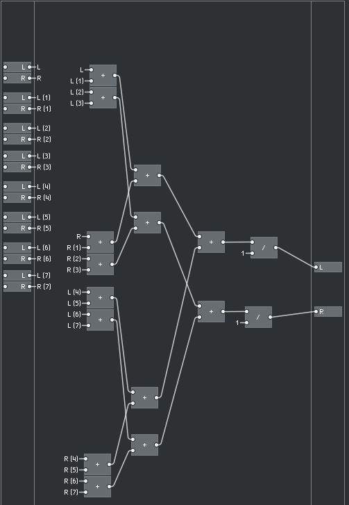
The summing macro is nothing special:
Core level macro
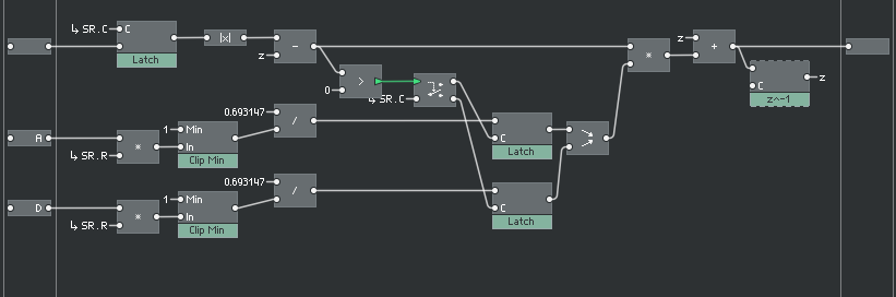
The level macro is a close copy of the original primary structure, and was built using the available library macros.
Let’s look more closely at how the envelope follower works. The envelope follower is fundamentally a low-pass filter running on the absolute value of the input signal. The gain of the low-pass is set by the attack and delay parameters, and the gain is chosen depending on a falling or rising value of the input signal.
Let’s model the equation in mathematica, and run it on a simple swelling sine wave.
inputWave =
  Table[Sin[2 Pi i/10000] Sin[2 Pi  i/100] // N, {i, 0, 5000}];
ListPlot[inputWave]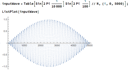
Manipulate[FoldList[Module[{
      x = Abs[#2] - #1,
      g
      },
     g = If[x > 0, 0.693147/attack, 0.693147/decay];
     #1 + g x
     ] &, 0.,
   inputWave] // (ListPlot[{inputWave, #}, ImageSize -> 500] &),
 {{attack, 50.}, 1., 1000.},
 {{decay, 100.}, 1., 1000.}]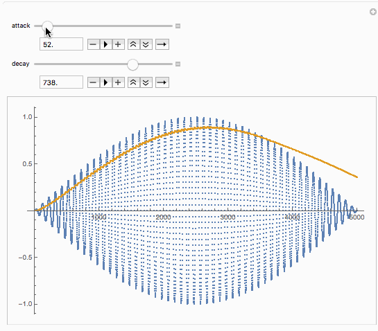
We can now piece together the puzzle. The computed waveform in Mathematica has a freaky start because the volume starts at absolute zero, which doesn’t seem to happen in reaktor (although you can get nasty pops when editing the ensemble, I haven’t looked closer into how to avoid these gain jumps in the envelope follower. Let’s use a slightly more eventful input waveform.
inputWave2 =
  Table[Sin[2 Pi i/10000] Sin[2 Pi  i/100] // N, {i, 0, 20000}];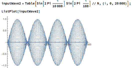
We can now see the compressor like effect of the level macro. The release value can be adjusted to make it subtler or more extreme.
envelopeFollow[input_, attack_, decay_] :=
 FoldList[Module[{
     x = Abs[#2] - #1,
     g
     },
    g = If[x > 0, 0.693147/attack, 0.693147/decay];
    #1 + g x
    ] &, 0., input];

Quiet@Module[{envelope = envelopeFollow[inputWave2, .1, 3000.]},
  ListPlot[{inputWave2, envelope, inputWave2/envelope[[2 ;;]]}]]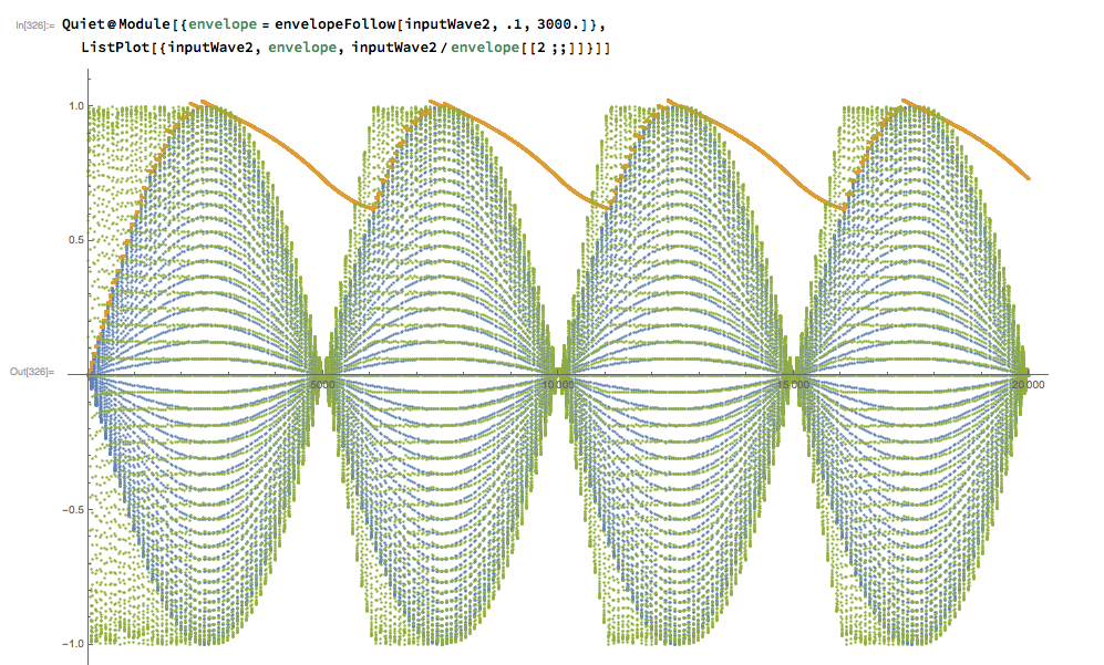
Core parameter computation
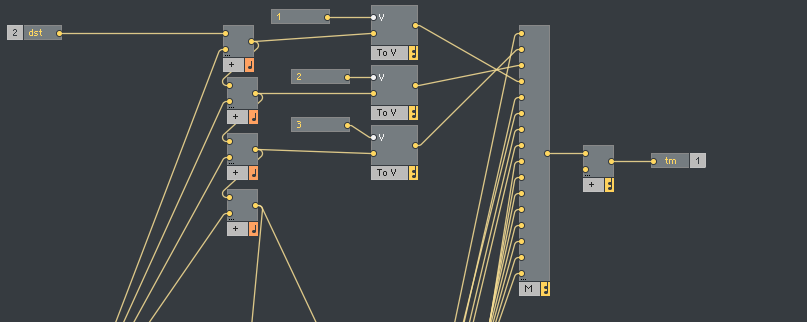
The computation of the delay line pitches is a simple implementation of the formulas above. Each delay line block is given an index input used to compute the spacing of the delay lengths.
Here is the asym computation:
And here is the delay length computation:
And we are almost done, the only missing part is the actual delay line, which is built using available library core cells.
Conclusion
This reverb is now available as a block in the user library for you to use. It is my first upload in 10 years, but Reaktor 6 and Reaktor Blocks really has me got back into patching. The great thing about Blocks is that you can patch while staying in a musical mindset, but it also allows you to very quickly integrate whatever nerdy DSP structures you come up with, and explore them on their own. This coupled to great UI resources and a vibrant community really make Reaktor stand out.
This was a fun exercise, and lazyfish’s ensemble are always amazing in their simplicity. This little exploration has led me to look up more resources about algorithmic reverbs, and I have started implementing a little zoo of different reverb topologies.
I hope to soon be able to upload a few more exploration into this fascinating topic.